Consensus: Making Transformers Less Fragile to Train

Abstract. A model's best training run tells us little about how easily we can reproduce that performance at a larger scale. We study consensus, a learned graph-based alternative to self-attention, across text, DNA, and protein transformers. Pure consensus preserves useful loss at learning rates where attention deteriorates, though attention can achieve a better tuned optimum. Hybrid models often retain attention's performance while reducing sensitivity, and experiments with query-key normalization show that the two approaches can complement one another. We connect these observations to measurements of loss curvature along optimizer updates.

You have enough compute to train a large model once. Before committing to the run, you train smaller models to choose the settings. You find a learning rate that works, scale up, and hope it still works.

How much room do you have to be wrong?

In one of our experiments, a 385M-parameter text transformer reaches a validation perplexity of about 43. Lower perplexity means the model assigns more probability to the held-out data. Perplexity is the exponential of negative log-likelihood (NLL), measured with natural logarithms: $\mathrm{PPL}=e^{\mathrm{NLL}}$ . Both are lower-is-better; a one-unit increase in NLL multiplies perplexity by about 2.72. The figures retain NLL, while the prose and tables use perplexity converted from the paper’s reported values. Double its learning rate, changing nothing else about the architecture, and perplexity rises to about 1,313. Training still produces a model. It is just a much worse one. The corresponding model built with consensus, our alternative to self-attention, moves from about 88 to 84.

Attention wins when it is well tuned. Consensus is much less sensitive to this change in the setting. For a team choosing how to spend a large training budget, both facts matter.

We first observed this behavior while developing Odyssey, our protein model. Consensus was designed to propagate information through local exchanges along a protein chain. Its tolerance of high learning rates raised a more general question: was this a consequence of the biological data, or had we changed something useful about transformer training?

To find out, we tested consensus across text, DNA, and joint protein sequence-and-structure models. The effect survives those changes of domain and objective. We also find that consensus and attention can work well in the same network, including when attention uses query-key normalization. The choice need not be between the best tuned model and the least fragile one.

How architecture affects training

The learning rate controls the size of an optimizer update. Too small, and the model learns slowly. Too large, and an update can overshoot the region where the loss would decrease. Between these extremes, the shape of the useful range depends on the model being trained.

A large-model program usually relies on transferring settings from cheaper experiments. Methods such as maximal-update parameterization make that transfer more principled. Yang et al., “Tuning Large Neural Networks via Zero-Shot Hyperparameter Transfer,” NeurIPS (2021). Warmup, Kalra and Barkeshli, “Why Warmup the Learning Rate? Underlying Mechanisms and Improvements,” NeurIPS (2024). normalization, Xiong et al., “On Layer Normalization in the Transformer Architecture,” ICML (2020). and gradient clipping also change which learning rates are usable. These address different parts of the optimization problem, rather than being interchangeable fixes. But the operation that moves information between tokens is itself part of the system being optimized. Changing it can change the training behavior.

Self-attention lets each token collect a weighted mixture of information from other positions. The weights depend on the current representations, allowing the network to make highly selective connections. Vaswani et al., “Attention Is All You Need,” NeurIPS (2017). The query-key scores pass through a softmax, so changes in their relative magnitudes can make the resulting weights more or less concentrated. Consensus also learns content-dependent interactions, but restricts their form: connected tokens exchange corrections that reduce selected differences between their representations.

This is a constraint on the computation inside a layer. Whether it makes the whole network easier to optimize is an empirical question. We can understand the constraint precisely, then test the complete trained models.

How consensus exchanges information

Imagine each token as a node in a graph. A node carries a vector of features, $u_i$ . An edge connects two nodes and measures their disagreement, $u_i-u_j$ . The edge then transforms that difference and contributes opposite corrections to the two endpoints.

The transformation is a learned positive-definite matrix:

R_{ij}=\alpha_{ij}I+\beta_{ij}\Lambda_{ij}^{\top}\Lambda_{ij}, \qquad \alpha_{ij},\beta_{ij}>0.

The scalar term couples all feature directions. The low-rank term chooses a small set of feature combinations for additional coupling. An edge can therefore reduce one kind of disagreement strongly and another weakly. Its behavior depends on the tokens it connects.

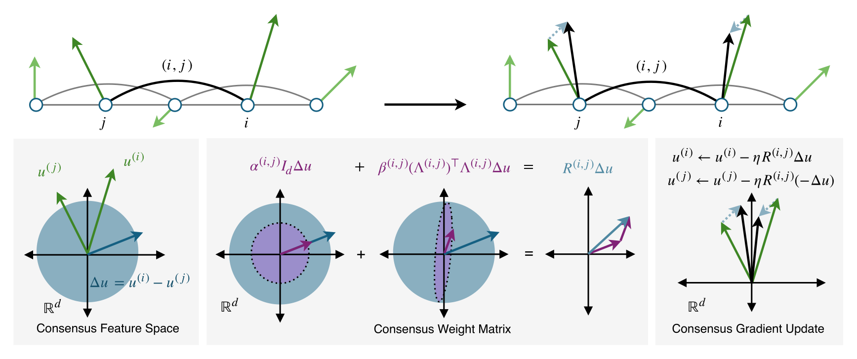
An edge transforms the difference between two node representations through scalar and low-rank components and applies opposite corrections to the endpoints. — One matrix-valued consensus exchange, from the paper. The learned edge matrix transforms the feature difference; both endpoints receive a correction. Contributions from all incident edges are accumulated before the node update.

For sequential data, we connect nearby positions in a sliding window. Most of the main experiments use two neighbors on either side. Local attention uses a similar connection pattern, but computes attention weights within the window; it gives us a way to test whether any observed advantage comes merely from locality. Beltagy, Peters, and Cohan, “Longformer: The Long-Document Transformer” (2020) develops sliding-window attention for long sequences. A shared graph does not imply a shared update rule.

To see what is special about the consensus update, strip away the learned matrices for a moment and give each node one scalar feature. On an undirected graph, define the energy as the sum of squared differences over edges:

E(u)=\sum_{\{i,j\}\in\mathcal E}(u_i-u_j)^2=u^\top Lu.

The graph Laplacian $L$ computes differences between a node and its neighbors. Taking a gradient step on this energy gives

u'=(I-2\eta L)u.

The update subtracts disagreement. A signal that alternates sharply between neighboring nodes changes more than one that varies gently along the graph. A constant signal does not change at all.

This is a low-pass filter on the graph. The figure below shows a simple numerical example: repeated updates suppress a rapidly varying component while changing the broad shape much less.

Three signal plots show scalar consensus suppressing rapid variation. A discrete frequency-response plot and component values show that after eight steps the constant is unchanged, the slow mode retains 98.17 percent of its amplitude, and the rapid mode retains 0.53 percent. — Scalar consensus on an unweighted 64-node path, with step size η = 0.12. Left: the input and its evolution under u⁽ᵏ⁾ = (I − 2ηL)ᵏu⁽⁰⁾, on identical axes. The input is uᵢ = 0.4 + cos(2π(i + ½)/64) + 0.45 cos(32π(i + ½)/64), for i = 0, …, 63. Right: amplitude multipliers (1 − 2ηλₘ)ᵏ at the path's 64 eigenvalues, λₘ = 2 − 2 cos(πm/64); markers denote the discrete modes, with lines connecting them. After eight steps, the slow component (m = 2) retains 98.17% of its amplitude and the rapid component (m = 32) retains 0.53%. The constant component is unchanged, so the mean remains 0.4. This is a computed illustration, not a trained-model result.

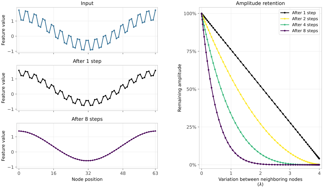
The learned matrix version makes this filtering selective and dependent on the input. It is not trying to turn a sentence or a protein into a constant vector. Projections, multiple heads, residual connections, and feed-forward layers transform and preserve information around the exchange. The filtering picture explains the core operation; it does not prove that every part of the network is contractive, or that its optimizer can never take a bad step.

From the energy to a matrix-valued update Aside

For each directed edge $(i,j)$ , let $R_{ij}=\alpha_{ij}I+\beta_{ij}\Lambda_{ij}^\top\Lambda_{ij}$ . The edge network predicts $\alpha$ , $\beta$ , and $\Lambda$ from the endpoint embeddings. Softplus makes the scalar coefficients positive; normalization controls the rows of the low-rank factor.

Holding these edge matrices fixed for the internal feature update, write

E(u)=\frac12\sum_{(i,j)\in\mathcal E} (u_i-u_j)^\top R_{ij}(u_i-u_j).

Differentiating includes both outgoing and incoming edges:

\nabla_{u_i}E= \sum_{j:(i,j)\in\mathcal E}R_{ij}(u_i-u_j) + \sum_{j:(j,i)\in\mathcal E}R_{ji}(u_i-u_j).

An implementation can accumulate these contributions without constructing a dense matrix. This pseudocode shows a single head, omitting positional transformations and the surrounding transformer block:

u = project_input(y)
grad = zeros_like(u)

for i, j in directed_edges:
    alpha, beta, Lambda = edge_parameters(y[i], y[j])
    delta = u[i] - u[j]
    correction = alpha * delta + beta * (Lambda.T @ (Lambda @ delta))
    grad[i] += correction
    grad[j] -= correction

output = project_output(u - eta * grad)

Updating both endpoints is essential. Two directed edges connecting the same pair may predict different matrices; each contributes its own quadratic cost.

For the spectral interpretation, stack node features and write the energy as $\tfrac12u^\top H_Eu$ , where

H_E=\mathcal B^\top\operatorname{diag}(R_e)\mathcal B\succeq0.

Here $\mathcal B$ is the graph incidence operator extended over feature dimensions. This formulation remains positive semidefinite even when opposite directed edges have different weights.

A uniform update multiplies an eigenmode by $1-\eta\lambda(H_E)$ . For the scalar energy in the main text, $H_E=2L$ , giving the factor $1-2\eta\lambda(L)$ . Under $0<\eta\leq1/(2\lambda_{\max}(L))$ , all scalar multipliers lie in $[0,1]$ : the operation attenuates without sign reversal. Larger steps can oscillate or become unstable.

The implementation learns its internal step sizes and includes rotary positional transformations. Those additions, as well as output projections and residual layers, fall outside this fixed-energy calculation. The optimizer learning rate $\alpha$ used to train the parameters is a different quantity from the internal consensus step $\eta$ .

Window size, information propagation, and compute Aside

A local graph makes communication cheap, but limits how far information can move in one layer. On an unweighted window-path graph with $N$ nodes and window radius $w$ , the paper bounds the first nonzero Laplacian eigenvalue:

2\sum_{j=1}^{w}\sin^2\!\left(\frac{\pi j}{2N}\right) \leq\lambda_1 \leq 4\sum_{j=1}^{w}\sin^2\!\left(\frac{\pi j}{2N}\right).

For the stated regime $w<N/2$ , these bounds give $\lambda_1=\Theta(w^3/N^2)$ . This eigenvalue controls the slowest nonconstant mode in the simple fixed-step filtering model. A larger window connects distant regions more effectively, though a stable step size also depends on the largest eigenvalue. Learned matrix weights require additional spectral bounds before the unweighted result can be transferred to them.

In the 193M text ablation, increasing $w$ from 2 to 12 improves validation perplexity from 94.5 to 74.7 without changing parameter count. It does increase work per layer. With width $d$ , edge rank $r$ , and edge-network hidden width $\xi$ , consensus costs

O\!\left(Nd^2+Ndwr(\xi+1)\right).

Linear dependence on length does not mean a faster implementation at every length. In the paper’s 54M text forward-pass benchmark on eight A40 GPUs, consensus runs at 2.43 iterations per second, MIX at 2.50, attention at 2.74, and sliding-window attention at 2.84. The present PyTorch implementation is slower in that setting. Kernel optimization is separate work.

Testing across text, DNA, and proteins

We compare four architectures in the main sweeps: standard self-attention (SA), self-consensus (SC), sliding-window attention (SW), and MIX, which uses attention in the first half of the layers and consensus in the second.

MIX tests a practical possibility. Attention may be especially useful for assembling information through direct, selective connections, without needing to perform every subsequent exchange. We can retain it in part of the network and ask whether consensus changes the resulting sensitivity.

The study spans three text sizes from 54M to 385M parameters, four DNA sizes from 51M to 1.1B, and three protein sizes from 35M to 320M. Text uses discrete diffusion; DNA and proteins use masked language modeling. This changes both the data and the objective under which we test the architecture. Text uses OpenWebText and the score-entropy objective of Lou, Meng, and Ermon, ICML (2024). DNA uses OpenGenome, introduced with Nguyen et al., “Sequence modeling and design from molecular to genome scale with Evo,” Science (2024). Protein data and tokenization follow Odyssey.

For each run, we evaluate the model on held-out data and separately score generated samples using a larger pretrained model. Validation perplexity measures the trained model’s predictions; external-model perplexity measures how predictable its generated samples are to the larger model. The external score helps reveal when a run produces samples that its own training loss does not adequately characterize. It is still another model’s judgment, not a measure of factual accuracy or biological function.

The text sweeps show the basic tradeoff. Attention reaches a good minimum, then deteriorates sharply as the learning rate rises. Consensus has a flatter response in the high-rate region, while MIX often remains close to attention near the minimum and performs better above it.

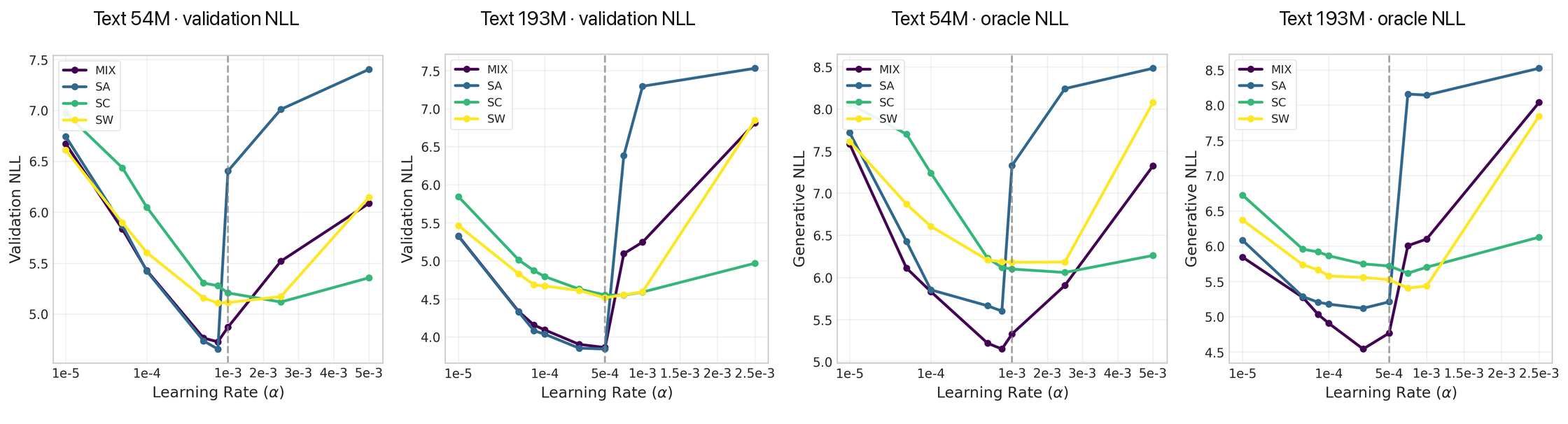
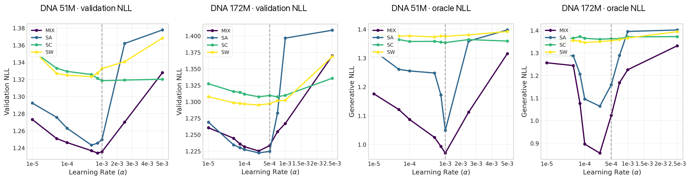
Text learning-rate sweeps at 54M and 193M parameters, showing held-out loss and GPT-2-Large scores of generated samples. — OpenWebText sweeps without warmup. The first two panels show validation NLL; the last two show GPT-2-Large NLL averaged over 1,000 generated samples. Attention's sharp high-rate deterioration is visible in both evaluations.

Changing to DNA preserves the broader high-rate validation range for consensus. The external-model curves are less uniform: an architecture’s advantage on held-out reconstruction need not translate into the same ordering of generated samples.

DNA learning-rate sweeps at 51M and 172M parameters, with held-out NLL and Evo2-1B NLL on generated sequences. — OpenGenome sweeps without warmup. Validation NLL appears first, followed by Evo2-1B NLL on 1,000 generated samples. Consensus's high-rate validation curves are flatter; the external-score advantage varies by panel.

For proteins, we evaluate amino-acid sequence and structure tokens separately. Both have to remain learnable for a joint model to be useful. The same qualitative pattern appears at 35M parameters and becomes particularly clear in the 133M validation curves.

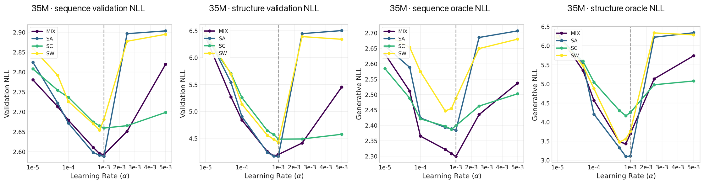
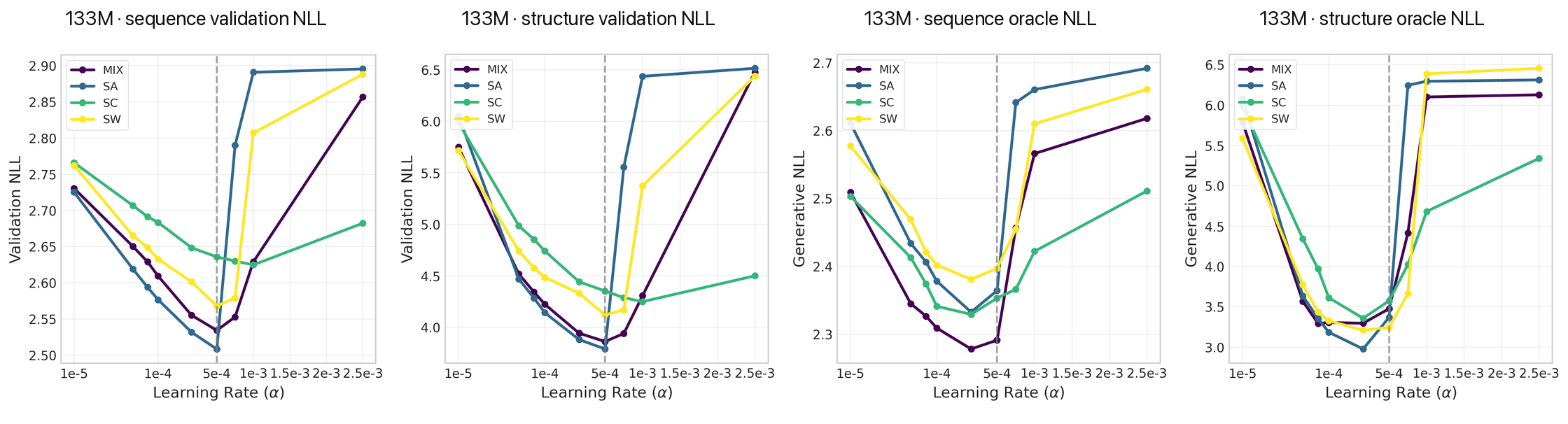
Sequence and structure learning-rate sweeps for 35M protein models, with separate validation and external-model scores. — 35M joint protein models without warmup. The first two panels measure held-out sequence and structure loss; the last two use Odyssey-1.2B to score generated samples.

Sequence and structure learning-rate sweeps for 133M protein models, showing consensus's broad high-rate validation range. — The same comparison at 133M parameters. Pure consensus retains useful validation loss through more of the high-rate sweep; MIX follows attention more closely near its best setting.

Sliding-window attention is an important control across these plots. Restricting attention to nearby positions does not reproduce consensus’s broad high-rate behavior. The result points toward the form of the update, rather than local connectivity alone.

The larger models make the tradeoff harder to ignore. In the 385M text example from the opening, MIX matches attention at the lower rate, but it too deteriorates when the rate doubles. Consensus tolerates the change while giving up considerable performance at the well-tuned setting.

385M text validation perplexity at two adjacent tested learning rates, without warmup. Values are converted from the paper's rounded NLL; underlines mark the best in each column, including ties at the reported precision.

Mechanism	LR 0.00025 (↓)	LR 0.0005 (↓)
Attention	43.4	1,312.9
Consensus	88.2	83.9
MIX (Attention + Consensus)	43.4	639.1

In the 320M protein experiment, the compromise is more favorable. At a learning rate of $5\times10^{-4}$ , MIX and attention reach similar structure perplexities, 42.7 and 40.9. At $7.5\times10^{-4}$ , MIX reaches 47.5 while attention deteriorates to 70.3. The sequence perplexities show the same ordering at the higher rate. Mixing the mechanisms can reduce sensitivity without paying the full performance cost of pure consensus, but the text result shows that it does not remove that sensitivity altogether.

What is controlled in these comparisons? Aside

All runs use pre-LayerNorm transformers, AdamW with weight decay 0.01, float32 precision, an effective batch size of 512, and global gradient-norm clipping at 1.0, on eight NVIDIA A40 GPUs. The main sweeps have no warmup; the additional comparisons below use 500 warmup steps.

Text 54M and DNA 51M/172M/331M runs use 5,000 global steps. Text 193M/385M runs use 20,000. Protein runs and DNA 1.1B runs use 3,000. We compare terminal checkpoints within each setting, not models trained to a common wall-clock budget.

Validation uses a 1% holdout from each dataset; for proteins, this comes from the AlphaFold DB subset. External NLL averages over 1,000 generations per model, using GPT-2-Large for text, Evo2-1B for DNA, and Odyssey-1.2B for proteins. The sampler unmasks one position at a time.

The protein comparison changes context conditioning as well as self-mixing: SA and SW use cross-attention, while SC and MIX use cross-consensus. It is therefore a comparison of those multitrack architectures, not an isolated replacement of one self-mixing operation. The text and DNA experiments help test whether the pattern extends beyond this particular multitrack setup.

Most consensus sweeps use $w=2$ , rank $r=4$ , and edge hidden width $\xi=256$ . Not every mechanism is tested at every scale. The paper’s full training matrix lists that coverage. The reported sweeps do not include repeated-seed confidence intervals; differences in curve shape are more informative here than tiny differences between individual minima.

Estimating the largest stable training step

The terminal losses tell us what happened. To investigate the dynamics, we ask a more local question: given the direction the optimizer is about to move, how large a step does the nearby loss surface permit?

Imagine walking downhill into a narrow valley. A short step lowers your altitude, but a longer step in the same direction can carry you up the opposite side. The gradient tells us which direction is downhill. Curvature tells us how quickly that direction stops being useful.

Let $\theta$ be the parameters, $v$ the optimizer’s update direction, and $\alpha$ the learning rate. A second-order expansion gives

\mathcal L(\theta+\alpha v)-\mathcal L(\theta) \approx \alpha\,g^\top v+\frac{\alpha^2}{2}v^\top Hv,

where $g$ is the gradient and $H$ the loss Hessian. For a downhill direction with positive curvature, the quadratic approximation predicts a decrease when

0<\alpha<\alpha_{\max}, \qquad \alpha_{\max}=-\frac{2g^\top v}{v^\top Hv}.

This is a directional estimate at a particular checkpoint and batch, not a global maximum learning rate for the network.

At the terminal checkpoint of the 133M protein model trained at $10^{-3}$ , all 25 measured consensus directions pass this local stability check. MIX passes 84%; attention and sliding-window attention pass none. Attention had passed 92% at the early checkpoint. The distinction develops during training, rather than being fully determined by the initial state.

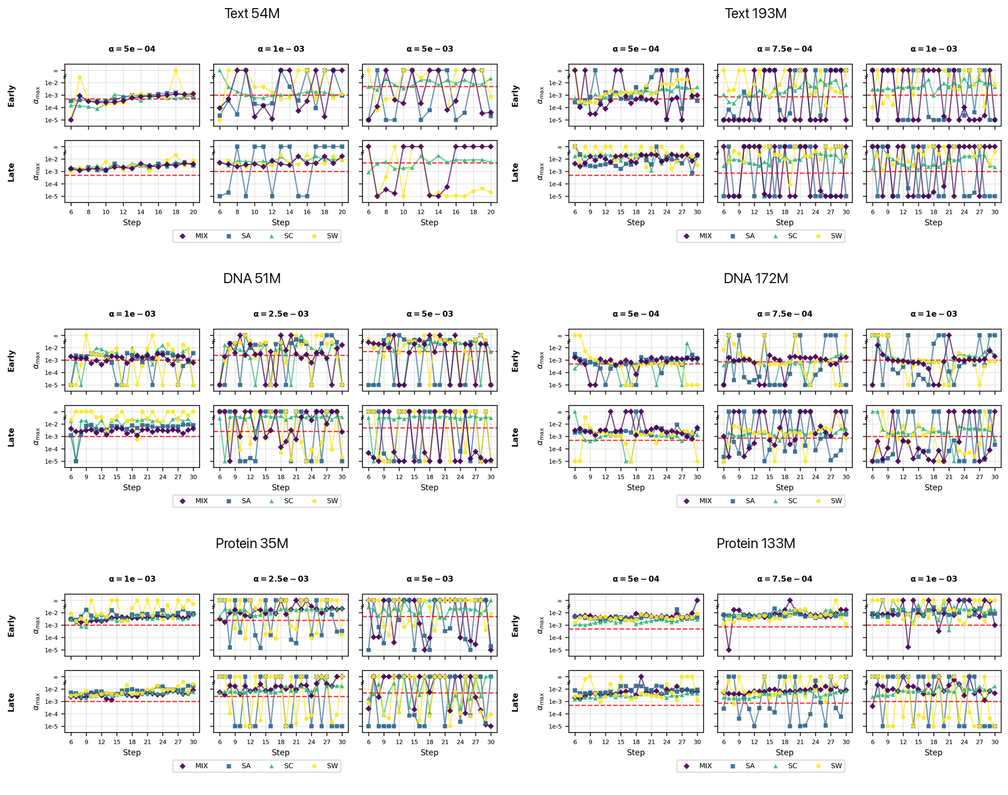
Early and terminal estimates of directional maximum stable learning rate across text, DNA, and protein models, compared with the training rate. — Directional stability measurements at early and terminal checkpoints. The red dashed line is the training learning rate; estimates above it pass the local quadratic check. Infinite estimates denote descending directions with negative curvature in the quadratic approximation.

The median finite estimate in that protein comparison is $6.8\times10^{-3}$ for consensus and $1.2\times10^{-6}$ for attention. Similar separations appear in text and DNA settings. The loss surfaces encountered by the trained architectures permit very different steps along their optimizer directions.

This helps connect architecture to the observed training behavior. It does not establish that the low-pass property alone causes the difference: the complete network, its learned parameters, and its optimizer all contribute. The useful finding is that changing the mixer changes both the terminal losses and these local measurements in a consistent direction across several settings.

Computing and interpreting the directional estimate Aside

Computing a full Hessian is unnecessary. We need only the scalar $v^\top Hv$ , obtained from a Hessian-vector product. For SGD, $v=-g$ , the expression simplifies to

\alpha_{\max} = \frac{2\|g\|^2}{g^\top Hg}.

For AdamW, the update direction also depends on moment estimates, preconditioning, clipping, and weight decay. The measurement therefore uses the optimizer direction, not just the raw gradient.

The protocol initializes Adam’s moments with five gradient batches, takes five warm steps, and then records 25 measured steps. Curvature batches contain 512 examples for the small models and 64 for the medium models. SA, SC, and MIX use autograd Hessian-vector products; SW uses a finite-difference estimate with $\epsilon=10^{-4}$ .

If the direction is uphill, the estimator assigns zero. For a descending direction with negative curvature, it assigns infinity because the quadratic term supplies no finite upper limit. Infinite estimates are omitted from finite medians. Higher-order terms still matter, so infinity is a convention of the approximation, not an actual stability guarantee.

The “stable fraction” is the fraction of those 25 measurements whose estimate exceeds the training rate. It is not a probability that a new training run will succeed, and the measurement directions use the stated moment-initialization procedure rather than the full optimizer history of the original run.

Combining consensus and attention

A practical architecture has to compete with the attention people would actually choose to use. Warmup is common, and attention itself can be modified to improve its behavior.

We therefore run additional comparisons with 500 steps of linear warmup, including gated attention and query-key-normalized attention. Query-key normalization changes the scale of the scores entering the attention softmax; Henry et al., “Query-Key Normalization for Transformers,” Findings of EMNLP (2020). gated attention adds learned control over its output. Qiu et al., “Gated Attention for Large Language Models: Non-linearity, Sparsity, and Attention-Sink-Free” (2025). We also test QK-MIX: query-key-normalized attention in the first half of the network and consensus in the second.

At 54M text parameters, normalized attention tolerates the high-rate settings much better than standard attention. QK-MIX combines that tolerance with stronger performance across the tested range. At a peak rate of $2.5\times10^{-3}$ , its validation perplexity is 90.0, compared with 107.8 for normalized attention, 138.4 for pure consensus, and 450.3 for standard attention.

The 1.1B DNA experiment tests the same combination at a larger scale. QK-MIX achieves the lowest validation perplexity at every tested learning rate. At the highest rate, it reduces perplexity by about 12% relative to normalized attention, from 3.78 to 3.32, and by about 9.5% relative to standard attention.

These differences can look small beside the text results. DNA prediction operates on a much smaller vocabulary: four canonical bases, rather than tens of thousands of text tokens. The DNA tokenizer also represents IUPAC ambiguity codes. Vocabulary, data, and evaluation objective all affect the scale of perplexity; absolute values should not be compared across the text and DNA tasks. The relative reduction is more informative than the size of the numerical gap.

DNA 1.1B validation perplexity after 500 warmup steps, at selected peak learning rates. Consensus uses window radius 4. Values are converted from the paper's rounded NLL; underlines mark the best in each column.

Mechanism	LR 0.0001 (↓)	LR 0.00025 (↓)	LR 0.0005 (↓)
Attention	3.39	3.49	3.67
Gated attention	3.53	3.39	3.39
Query-key normalized attention	3.74	3.78	3.78
Consensus	3.60	3.60	3.56
MIX (Attention + Consensus)	3.42	3.42	3.63
QK-MIX (Normalized attention + Consensus)	3.35	3.35	3.32

To put the per-base scale in perspective, consider a hypothetical 1,000-base gene. Suppose a model predicting one base at a time maintained the average negative log-likelihoods from the highest-rate comparison: 1.33 for normalized attention and 1.20 for QK-MIX. Over those 1,000 predictions, the improvement would accumulate to 130 nats, or about 188 bits. In this idealized sequence-coding interpretation, that is a roughly 9.8% reduction in the description length of the same gene. For a sequential model, negative log-probabilities add across positions. Using the paper’s rounded values, the illustrative difference is $1{,}000\times(1.33-1.20)=130$ nats, or $130/\ln 2\approx188$ bits. The 9.8% reduction in this logarithmic quantity differs from the perplexity reduction, $1-e^{1.20-1.33}\approx12.2\%$ .

This is an illustration of how per-base improvements accumulate, not a measured whole-gene likelihood or compression result.

The measured result is that consensus contributes alongside normalized attention with warmup enabled. Neither normalization nor pure consensus is the strongest model in this DNA sweep, but their hybrid wins at every tested rate. The components can be useful together in ways that their isolated performance would not suggest.

These follow-up runs use larger consensus windows than the main sweeps, $w=8$ for text and $w=4$ for DNA. They establish the behavior of those warmup-equipped configurations; they do not isolate the effect of adding warmup alone.

What this means for larger models

The usual architecture comparison asks which model achieves the lowest loss after tuning. We think it should also ask how the result changes when the training recipe is slightly wrong. At scale, that sensitivity affects how much we can learn from small experiments before committing to expensive ones.

Consensus gives us a concrete way to study that second question. Its disagreement-reducing update has a different high-rate response from attention across several domains. Pure consensus reveals the tradeoff most clearly; hybrids show that some of the tolerance can coexist with attention’s performance. Normalization and consensus can also complement one another, rather than competing to solve the entire problem separately.

The next step is to test those combinations in longer, larger training runs and determine how reliably their settings transfer from small proxies. That would connect the sensitivity measured here to the decision that motivated the work: how confidently can we choose the recipe before committing to the run?

This question came out of building a protein model. Its answer need not stay inside protein modeling. A lab trying to build more capable biological tools should be prepared to improve the learning machinery as well as the data it learns from.

The paper includes the full sweeps, derivations, and training configurations. The implementation is available on GitHub.