Odyssey: Scaling Novel Primitives for Better Protein Models

Suppose you know what a small part of a protein needs to look like. A few amino acids have to sit at particular angles and distances from one another to perform a chemical reaction. You want to keep those residues, keep their arrangement, and build a new protein around them.

This sounds like a request for the rest of a sequence. But most of the request is geometric. The new chain has to fold into a shape that holds the specified residues in place. The residues surrounding them have to be compatible with that shape. And changing one part of the chain can change what is possible elsewhere. You are designing the sequence and the structure, whether or not your model represents both.

At Anthrogen, we want to design proteins that do things we cannot yet ask biology to do reliably. That requires models we can give increasingly precise instructions, including instructions about the physical object we want to build. Odyssey is our first model family built toward that goal. We revisit two basic choices: how information moves through the network, and what the network learns to predict. A new mechanism called consensus exchanges information along the chain. Discrete diffusion learns to complete sequence and structure jointly, progressively filling in missing parts while conditioning on what is known.

We trained models with 1.2B, 12B, and 102B parameters. The largest run used $1.1\times10^{23}$ FLOPs. The work here is computational: the architecture, its scaling behavior, and an initial experiment in teaching the model to prefer designs according to a specified structural objective. These are the modeling decisions we intend to build on as our experimental program develops.

Modeling sequence and structure together

Treating amino acids as tokens has been extraordinarily productive. Protein language models learn structural and functional information from sequences alone, without being explicitly taught either. Rives et al., “Biological structure and function emerge from scaling unsupervised learning to 250 million protein sequences,” PNAS (2021). But a sequence-only model cannot receive the geometric part of our request directly. We need a representation in which both amino-acid identity and structure can be supplied, hidden, or generated.

Protein generation has developed along several paths. ProGen generates amino-acid sequences autoregressively; Madani et al., “Large language models generate functional protein sequences across diverse families,” Nature Biotechnology (2023). DPLM learns sequence generation through discrete diffusion; Wang et al., “Diffusion Language Models Are Versatile Protein Learners,” ICML (2024). RFdiffusion generates protein backbones by denoising spatial coordinates. Watson et al., “De novo design of protein structure and function with RFdiffusion,” Nature (2023). More recent models, including ESM3 Hayes et al., “Simulating 500 million years of evolution with a language model,” Science (2025). and DPLM-2, Wang et al., “DPLM-2: A Multimodal Diffusion Protein Language Model” (2024). bring sequence and structure into a shared discrete representation. Joint modeling is still young, and representing both modalities leaves the architecture and training objective far from settled.

Odyssey gives each residue two tokens: one for its amino acid and one for its structure. The structure token comes from an encoder that compresses atomic coordinates into a discrete vocabulary. A decoder converts the completed structure tokens, together with the sequence, back into coordinates. Between those two operations, the model works with two aligned streams of symbols.

Our contribution is in the primitives operating on those symbols. We replace self-attention in the residue-processing layers with learned local consensus, and train joint generation with a continuous-time, score-entropy diffusion objective. These choices change both how the model propagates information and how it learns to generate a protein. We study their behavior in controlled experiments and scale the resulting architecture to 102B parameters.

The inputs also include context. Secondary structure, solvent accessibility, domain annotations, and structure-prediction confidence describe individual residues or regions. Evolutionary group assignments and text descriptions describe the protein more broadly. We treat these as conditioning information, rather than requiring the model to generate every annotation whenever it designs a protein.

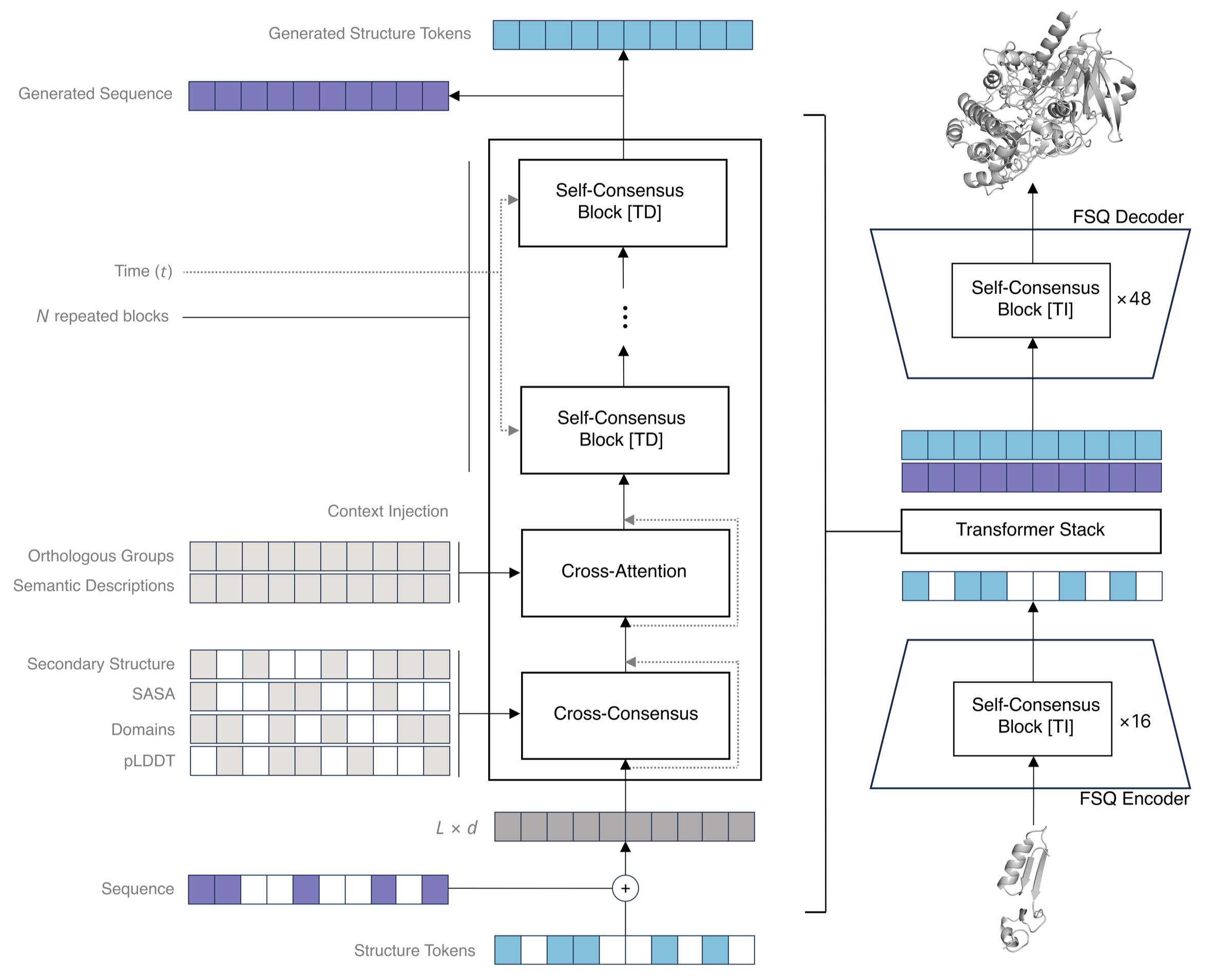
This distinction lets us keep a single model while changing the design problem. For backbone-conditioned sequence design, supply structure and hide sequence. For local repair, hide a region of both tracks. For the enzyme example, preserve the catalytic residues and their geometry and ask the model to complete the surrounding chain. The prompt specifies what is fixed; the model supplies what is missing.

Training data and what counts as a distinct protein Aside

Our source collection contains approximately 3.66 billion records from sequence and structure databases, including UniRef, SRC, MERC, AntiRef, OMG, the PDB, ESM Atlas, Lin et al., “Evolutionary-scale prediction of atomic-level protein structure with a language model,” Science (2023). and AlphaFold DB. Jumper et al., “Highly accurate protein structure prediction with AlphaFold,” Nature (2021). Predicted structures supply training information, not experimental confirmation. That is a source-record count, not a claim of 3.66 billion unrelated proteins. Closely related sequences are common within and across these resources. The data sources and counts are listed in Supplementary Table S1.

We cluster most sequence sources first at 90% identity and then at 60%. Sampling a 60%-identity cluster with weight $n/(1+\log n)$, where $n$ is its size, reduces the dominance of large families without giving every rare cluster the same weight as a common one. We then sample a representative from its finer clusters. Antibody sources use tighter thresholds, 98% and 92%; PDB records use 100% and 60%. The structure tokenizer uses a separate 40%-identity clustering procedure.

The sequence cutoff is January 1, 2024, and the structure cutoff is August 1, 2022. These cutoffs matter for evaluating later structures without having trained on their deposited coordinates. They do not establish that every evaluation protein lacks a related sequence in training.

The eight input tracks comprise two source tracks and six context tracks. Models support 2,046 content residues, with the remaining two positions reserved for boundary tokens.

Local communication through consensus

A protein chain imposes a particular kind of dependence. Two residues far apart in sequence can meet in the folded structure, but the chain between them must also fit. Bringing those two positions together constrains everything connecting them. This suggests learning how local compatibility propagates, rather than assuming every residue needs a direct connection to every other residue in every layer.

Standard self-attention provides those direct connections. It scores pairs of tokens and uses the scores to mix information across the sequence. Vaswani et al., “Attention Is All You Need,” NeurIPS (2017). For a fixed model width, the all-pairs interaction has quadratic cost in sequence length. Consensus instead connects nearby residues along the sequence. Each edge computes a difference between the two representations and learns which components of that difference to reduce. Repeating the operation through depth lets information travel farther along the chain.

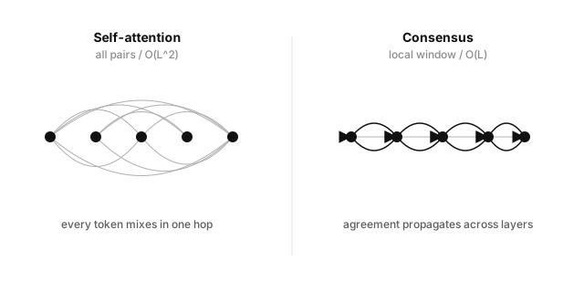
The word “agreement” can make the operation sound like averaging. It is more selective than that. A learned matrix on each edge determines which feature directions should be coupled strongly. For representations $u_i$ and $u_j$, the edge assigns a disagreement cost

$$E_{ij}=\frac12(u_i-u_j)^\top R_{ij}(u_i-u_j), \qquad R_{ij}=\alpha_{ij}I+\beta_{ij}\Lambda_{ij}^\top\Lambda_{ij}.$$

Here $\alpha_{ij}$ and $\beta_{ij}$ are positive learned scalars. $\Lambda_{ij}$ selects a low-dimensional set of feature combinations for additional coupling. Consensus updates the endpoint representations in the direction that reduces the sum of these costs. The network learns what should agree, not just how much to average.

This gives us a local operation whose cost grows linearly with sequence length at fixed width and window size. We use it both to mix residues and to incorporate residue-aligned context. We retain cross-attention for text and evolutionary context, where there is no corresponding position on the chain.

The locality is a modeling choice, not a claim that proteins have only local interactions. It trades immediate all-pairs access for repeated local communication. Whether that trade is useful has to be established by training the model.

The consensus update and its contraction conditions Aside

For a fixed input, let $\mathcal E$ contain the directed edges between positions with $0<|i-j|\leq w$. Hold their learned matrices fixed while taking the internal energy gradient:

$$E(u)=\frac12\sum_{(i,j)\in\mathcal E} (u_i-u_j)^\top R_{ij}(u_i-u_j).$$

Every edge contributes at both endpoints. Consequently,

$$g_i= \sum_{j:(i,j)\in\mathcal E}R_{ij}(u_i-u_j) + \sum_{j:(j,i)\in\mathcal E}R_{ji}(u_i-u_j), \qquad u_i'=u_i-\eta_i g_i.$$

The incoming term matters: the model need not predict the same matrix for $(i,j)$ and $(j,i)$. Omitting it would no longer give the gradient of the stated energy.

Stacking the representations into $u$ gives $E(u)=\tfrac12u^\top H_Eu$ with $H_E$ positive semidefinite. For a uniform internal step $\eta$, an eigenmode with eigenvalue $\lambda$ is multiplied by $1-\eta\lambda$. With $0<\eta\leq1/\lambda_{\max}(H_E)$, all these multipliers lie between zero and one. Differences are attenuated without reversing their sign.

This is the fixed-matrix, unpositioned core. The implemented block includes learned node-dependent steps, rotary position transformations, output projections, residual connections, and an MLP. The complete network is not covered by that simple contraction argument. In particular, $\eta$ is an internal feature-update size, not the optimizer learning rate.

For length $L$, model width $d$, window $w$, edge rank $r$, and edge-network hidden width $\xi$, the reported block complexity is

$$O\!\left(Ld^2+Ldwr(\xi+1)\right).$$

The dependence on $L$ is linear when the other quantities are fixed. This is an asymptotic statement; it does not establish a wall-clock speed advantage over optimized attention kernels.

Encoding protein structure

The structure tokens have to preserve enough geometry to make all of this worthwhile. A compact vocabulary that loses the arrangement we wanted to keep would defeat the point.

We use finite scalar quantization, or FSQ. An encoder maps each residue’s backbone geometry into five learned latent coordinates. Each coordinate is rounded to one of a fixed set of values: seven possibilities on one axis and five on each of the other four. The resulting vocabulary has $7\times5^4=4{,}375$ entries. Mentzer et al., “Finite Scalar Quantization: VQ-VAE Made Simple,” ICLR (2024). FSQ replaces a learned vector codebook with a fixed product of scalar levels. The learned encoder decides how to use those levels. These are coordinates in a learned representation, not a grid onto which we snap the protein’s atoms.

We train the encoder to preserve the backbone first. Then we freeze it and train a larger, sequence-conditioned decoder to reconstruct the backbone and side-chain heavy atoms. The separation is deliberate: amino-acid identity determines which side-chain atoms exist, while the structure vocabulary should encode geometry without using a residue’s atom layout as a shortcut to its identity.

We evaluate reconstruction on CAMEO, CASP15, and CASP16 structures collected after the tokenizer’s structural training cutoff. RMSD measures the average spatial error after alignment; lower is better. The comparison below asks how much backbone accuracy survives the second training stage and how accurately the decoder recovers the fuller atomic representation.

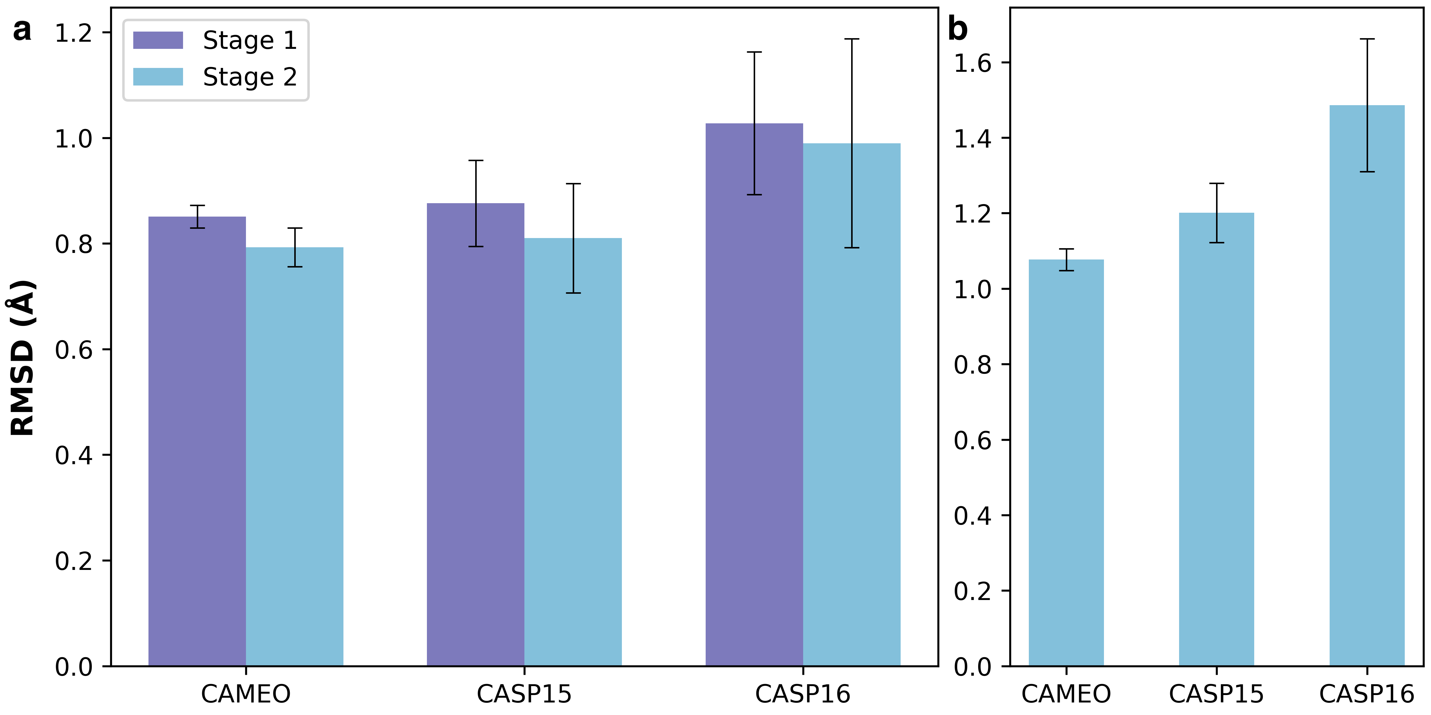
The aggregate results show that the small structure vocabulary retains substantial geometric information. Individual reconstructions also show what the averages hide: local errors, changes in the relative placement of regions, and occasional large failures. The archived examples below include both close overlays and reconstructions with substantial disagreement.

1. 7YLD chain E · 84 residues · Backbone RMSD 1.35 Å

2. 8F9Q chain A · 495 residues · Backbone RMSD 1.97 Å

3. 8GAC chain A · 103 residues · Backbone RMSD 1.00 Å

4. 8J2S chain B · 460 residues · Backbone RMSD 1.50 Å

5. 8J5F chain A · 238 residues · Backbone RMSD 2.19 Å

6. 8K4M chain A · 124 residues · Backbone RMSD 11.37 Å

7. 8QPM chain A · 329 residues · Backbone RMSD 0.48 Å

8. 8R8O chain A · 262 residues · Backbone RMSD 3.56 Å

9. 8RZ1 chain A · 228 residues · Backbone RMSD 17.76 Å

10. 8SOW chain C · 219 residues · Backbone RMSD 17.52 Å

11. 8T6C chain A · 119 residues · Backbone RMSD 1.01 Å

12. 8ZB3 chain A · 290 residues · Backbone RMSD 1.71 Å

13. 9GN3 chain C · 298 residues · Backbone RMSD 4.87 Å

14. 9I2L chain A · 260 residues · Backbone RMSD 4.30 Å

15. 9JWA chain B · 203 residues · Backbone RMSD 2.78 Å

1 of 15

Why train the tokenizer in two stages? Aside

The first stage trains a roughly 50M-parameter encoder-decoder on the three backbone atoms N, Cα, and C. We expose it to masked coordinates so that partially specified structures are familiar inputs. Reconstruction loss is evaluated at observed positions: the tokenizer is not itself trained to invent the missing protein.

The second stage freezes the encoder and trains a roughly 500M-parameter decoder on complete structure tokens and sequence. It outputs atom-14 coordinates, a residue-dependent representation with up to 14 heavy atoms. Sequence tells the decoder which atoms occupy the available slots. A glycine and a tryptophan do not come with the same parts list.

We align reconstructed and target coordinates before computing the error. The fit uses a proper rotation, with determinant $+1$, rather than allowing a reflection. Kabsch, “A solution for the best rotation to relate two sets of vectors,” Acta Crystallographica A (1976). Allowing reflections would let a mirror image receive a misleadingly good fit.

This division lets the generative model operate over a compact backbone representation while leaving sequence-dependent atomic reconstruction to a separate decoder. Its reconstruction errors still matter downstream: a token constraint is only as faithful as its encoding and decoding.

Learning to generate with diffusion

Once sequence and structure share a discrete representation, we can train on incomplete versions of both. But “incomplete” covers very different problems. Recovering a few amino acids from an otherwise visible protein is much easier than building most of a chain around a small fixed site. We want the training objective to describe how to move between different amounts of missing information.

In discrete diffusion, the forward process replaces content tokens with a special MASK token. Later times correspond to more corruption. The model receives the corrupted protein and the time, and learns the reverse process: replacing masks with compatible sequence and structure tokens. Our objective follows Lou, Meng, and Ermon, “Discrete Diffusion Modeling by Estimating the Ratios of the Data Distribution,” ICML (2024), which introduces score entropy for learning discrete reverse-time dynamics. Generation proceeds by unmasking, with visible constraints held fixed.

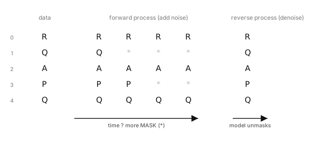
The difference from masked language modeling is not simply that we hide more tokens. A masked model learns to predict hidden tokens under a chosen corruption distribution. A diffusion model learns the reverse dynamics of a specified corruption process, with a time-dependent objective tied to the likelihood of the generated data. Variable masking already appears in models such as ESM3; we compare against it as well as the familiar fixed 15% setting. The 15% convention comes from Devlin et al., “BERT: Pre-training of Deep Bidirectional Transformers for Language Understanding,” NAACL (2019). Our variable-masking baseline uses ESM3’s betalinear30 schedule for sequence and cosine schedule for structure.

We train all three objectives with consensus at 35M, 142M, and 1.2B parameters. For this comparison, diffusion spans masking probabilities from 0% to 100%, and all models are evaluated under variable corruption. The diffusion models reach lower reported validation scores in the plots; the 1.2B fixed-mask model also shows pronounced overfitting.

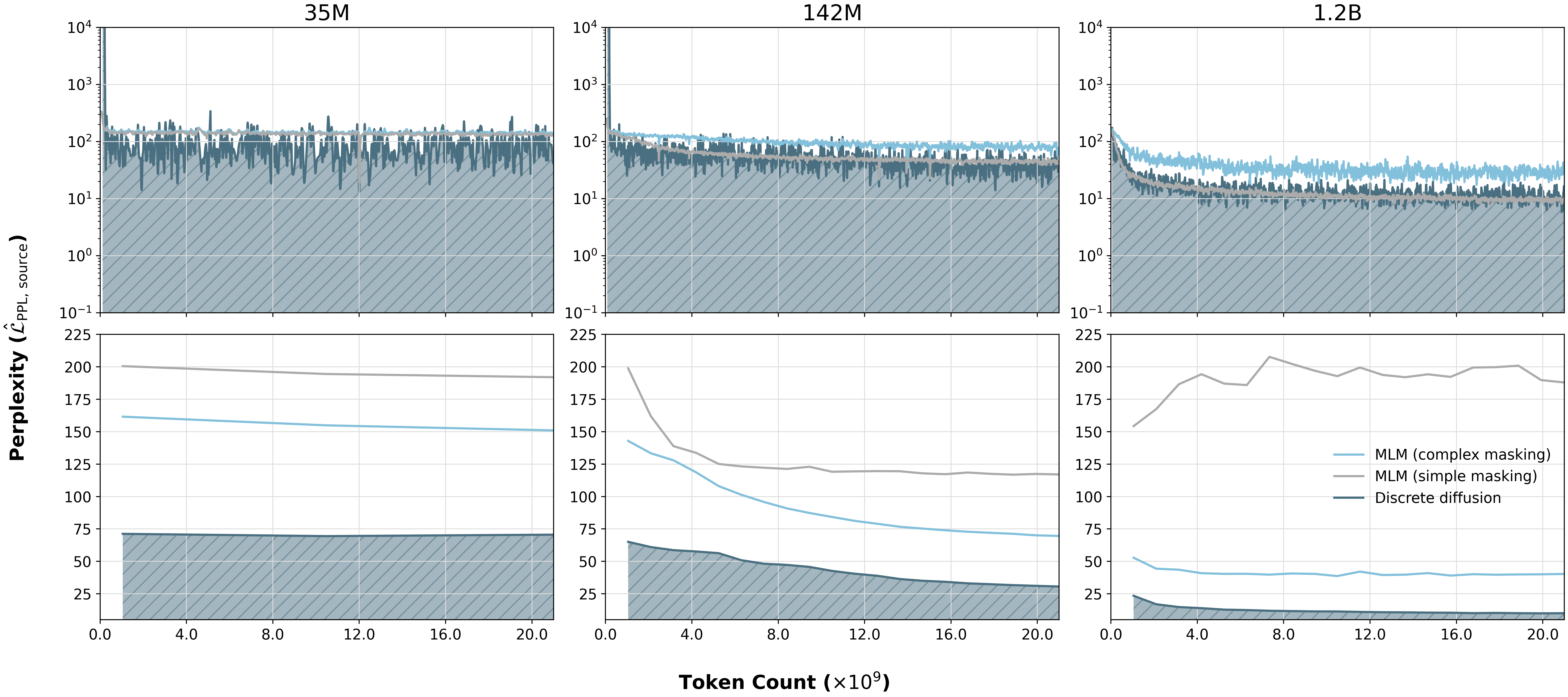
That last distinction matters when reading the vertical axis. The diffusion objective bounds a joint generative likelihood; the masked objectives score conditional reconstruction. Their numerical values are not interchangeable measurements of a single likelihood. The comparison supports training across the corruption levels needed for completion, but it does not establish a precise likelihood advantage over the masked models.

For the production models, we use a different schedule, chosen for conditional design: the maximum expected masking fraction is about 84%. The objective can describe almost fully masked inputs, but the schedule determines how much of that regime a particular model sees.

The reverse process, noise schedule, and likelihood bound Aside

Write the cumulative corruption rate as $\bar\sigma(t)=\int_0^t\sigma(s)\,ds$. An ordinary content token survives to time $t$ with probability

$$q_t=\exp[-\bar\sigma(t)].$$

Otherwise it becomes MASK. Context tracks use IGN to represent missing conditioning information. Boundary and padding tokens do not participate in corruption.

For two joint token states $z$ and $z'$ differing at one position, the reverse transition rate depends on a probability ratio. With the convention that $Q_t(z',z)$ is the forward rate from $z'$ to $z$,

$$\widehat Q_{T-t}(z,z') = Q_t(z',z)\frac{p_t(z')}{p_t(z)}.$$

The network learns the ratio. Forward corruption acts independently at each position, but reversal depends on the whole visible protein, so independent masking does not imply independent generation.

Production and scaling runs use the geometric rate $\sigma(t)=\sigma_{\min}(\sigma_{\max}/\sigma_{\min})^{t/T}$, with $\sigma_{\min}=0.31$ and $\sigma_{\max}=5.68$. At the endpoint, $\bar\sigma(T)\approx1.847$ and $q_T\approx0.158$. The diffusion-versus-MLM ablation instead uses a linear masking-probability schedule over the full range. These experiments should not be read as using identical corruption distributions.

The finite terminal survival probability also affects likelihood reporting. The bound takes the form

$$-\log p_\theta(z_0) \leq \mathcal L_{\mathrm{DWDSE}}(z_0) + D_{\mathrm{KL}}\!\left(q_T(\cdot\mid z_0)\,\|\,\pi_T\right),$$

where DWDSE is diffusion-weighted denoising score entropy and $\pi_T$ is the generation prior. A strictly all-MASK prior would assign zero probability to terminal states that still contain content. The paper therefore uses a prior with nonzero content support and includes the resulting correction. Exponentiating the denoising loss alone does not give the production models’ perplexity bound.

Scaling and training stability

A new architecture needs more than a promising small run. We need to know how additional parameters and training data affect it, and whether we can train a large instance without making its performance depend on an exceptionally narrow choice of settings.

We first trained a scaling sweep from 142M to 1.2B parameters, using up to 80B tokens. We fit the relationship between validation loss, model size, and data, then used the fit to plan the larger runs. This follows the compute-allocation question studied in language-model scaling: with a fixed budget, how much should go into a larger model and how much into training it longer? Kaplan et al., “Scaling Laws for Neural Language Models” (2020). Hoffmann et al., “Training Compute-Optimal Large Language Models,” NeurIPS (2022). A scaling relationship is specific to the model, data, and training procedure being measured; importing another model’s fit would skip the experiment.

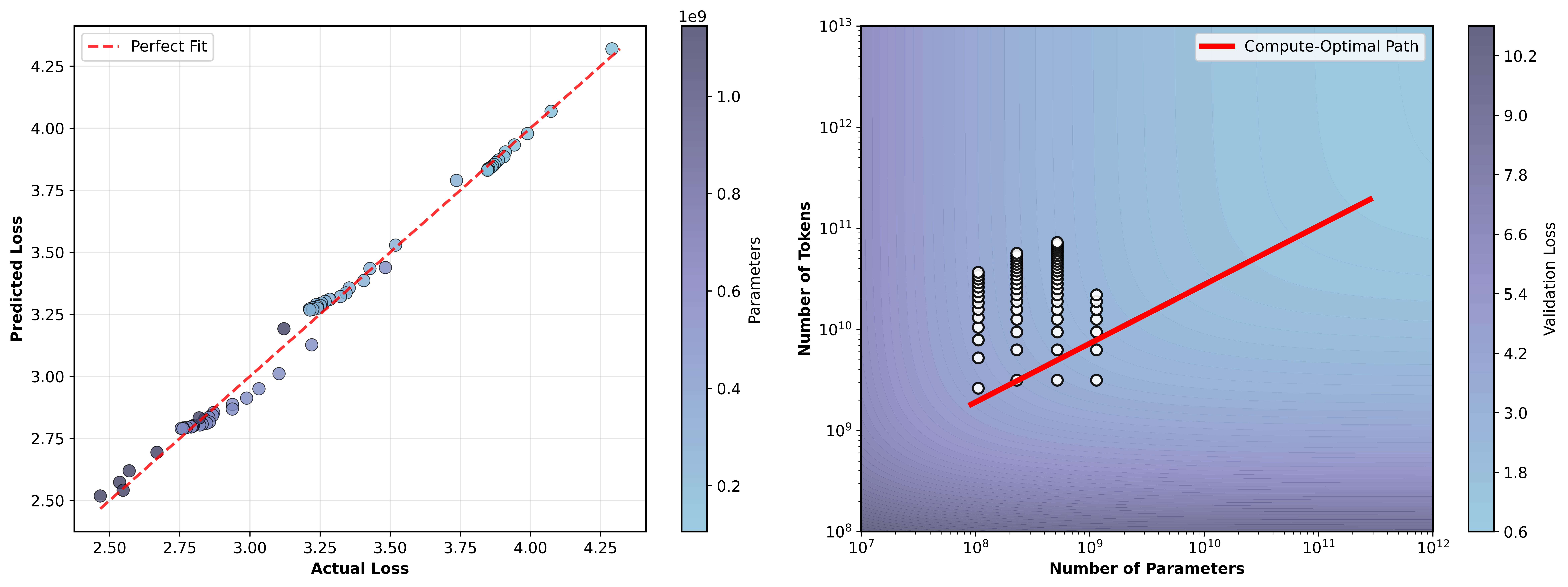
At our largest compute budget, the fit predicted an optimum around 142B parameters. We trained 102B within the available resources. That is a substantial extrapolation from the sweep, so we treat the fit as a planning tool and report the larger models’ measured losses separately.

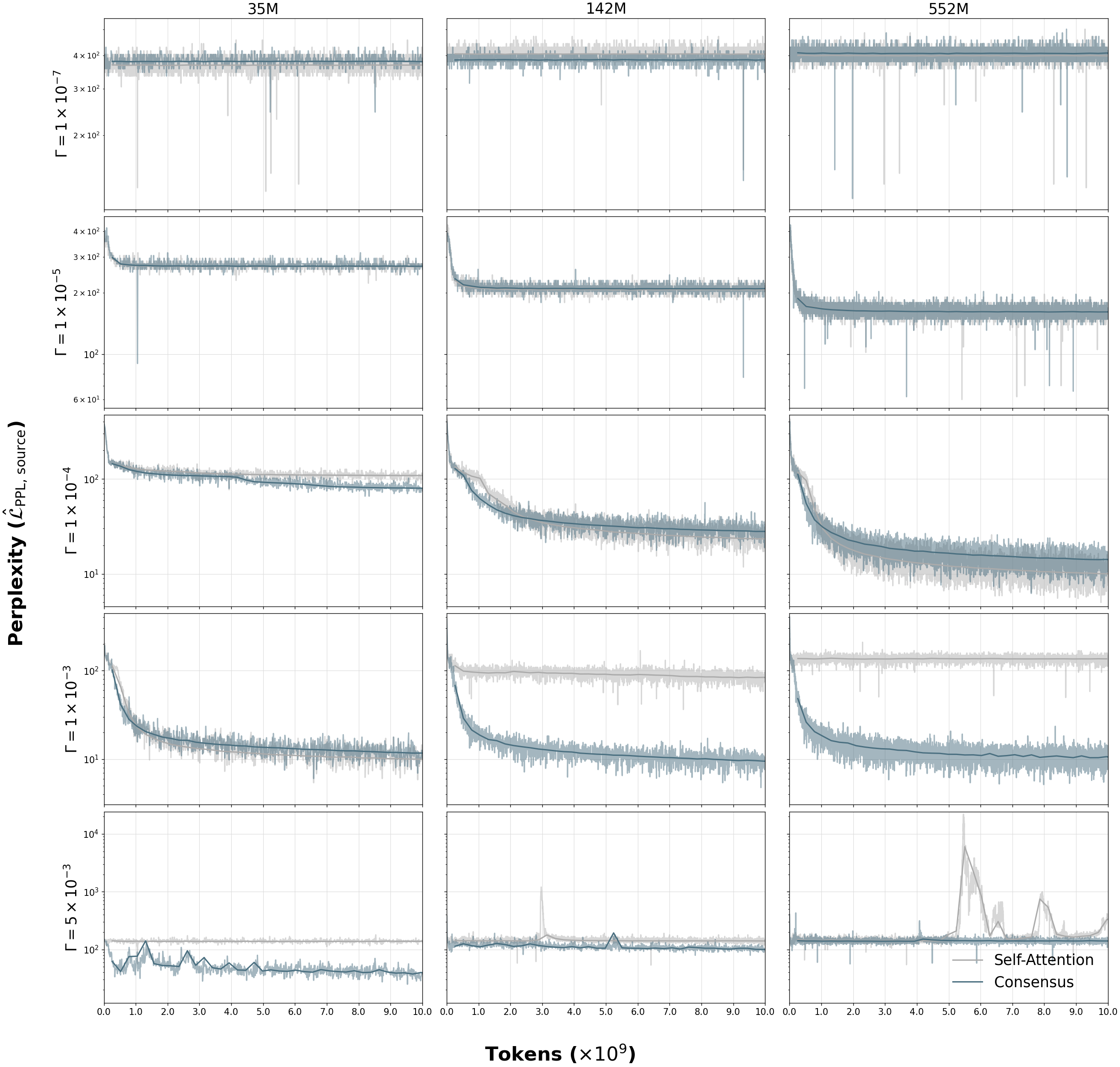
We also tested sensitivity to the optimizer learning rate. In same-scale masked-model comparisons, consensus continued to learn at rates where attention performed poorly, with the difference becoming more pronounced at larger sizes. This matters because tuning every choice at full scale is expensive. A model that tolerates a wider range of rates gives us more room for the settings chosen in smaller experiments to transfer.

The production family then gives us a direct check on scale: validation denoising loss decreases at each size, from 1.987 to 1.629 to 1.356. Both sequence and structure scores improve. The table includes the terminal-prior correction needed to turn those losses into reported perplexity upper bounds.

Parameters	Validation DWDSE	Perplexity upper bound
1.2B	1.987	≤18.218
12B	1.629	≤12.730
102B	1.356	≤9.696

The learning-rate observation also raised a question beyond protein modeling: does consensus make transformer training less sensitive to the learning rate in other domains? We investigate that separately in our consensus release, with text and DNA as well as proteins.

Aligning the model for enzyme design

Pretraining learns the patterns present in protein data. A design task adds a preference: among plausible proteins, which ones better satisfy the requirement? A protein that looks typical is not necessarily the protein we need.

We test whether the 1.2B model can learn a computational preference for six enzyme-design tasks. For each task, we preserve catalytic residue identities and geometry, generate candidate scaffolds, predict their folded structures, and score two properties: confidence in the overall fold and agreement with the requested active-site geometry.

The score combines pTM, a structure predictor’s global fold-confidence measure, with catalytic-site RMSD, or cRMSD, which measures deviation from the target geometry. We use the score to form pairs of preferred and less-preferred candidates, then align the model with D2-DPO, Borso et al., “Preference-Based Alignment of Discrete Diffusion Models” (2025). a diffusion-specific form of direct preference optimization. Rafailov et al., “Direct Preference Optimization: Your Language Model is Secretly a Reward Model,” NeurIPS (2023). Preferences need not come from human ratings; here they come from a computational design objective.

After alignment, the model’s internal scores are positively correlated with that objective on all six tasks. For 1CWY, the reported Spearman rank correlation moves from $-0.265$ to $0.654$; for 1BS9, from $0.090$ to $0.792$. The model has learned an ordering that better agrees with the preference we supplied.

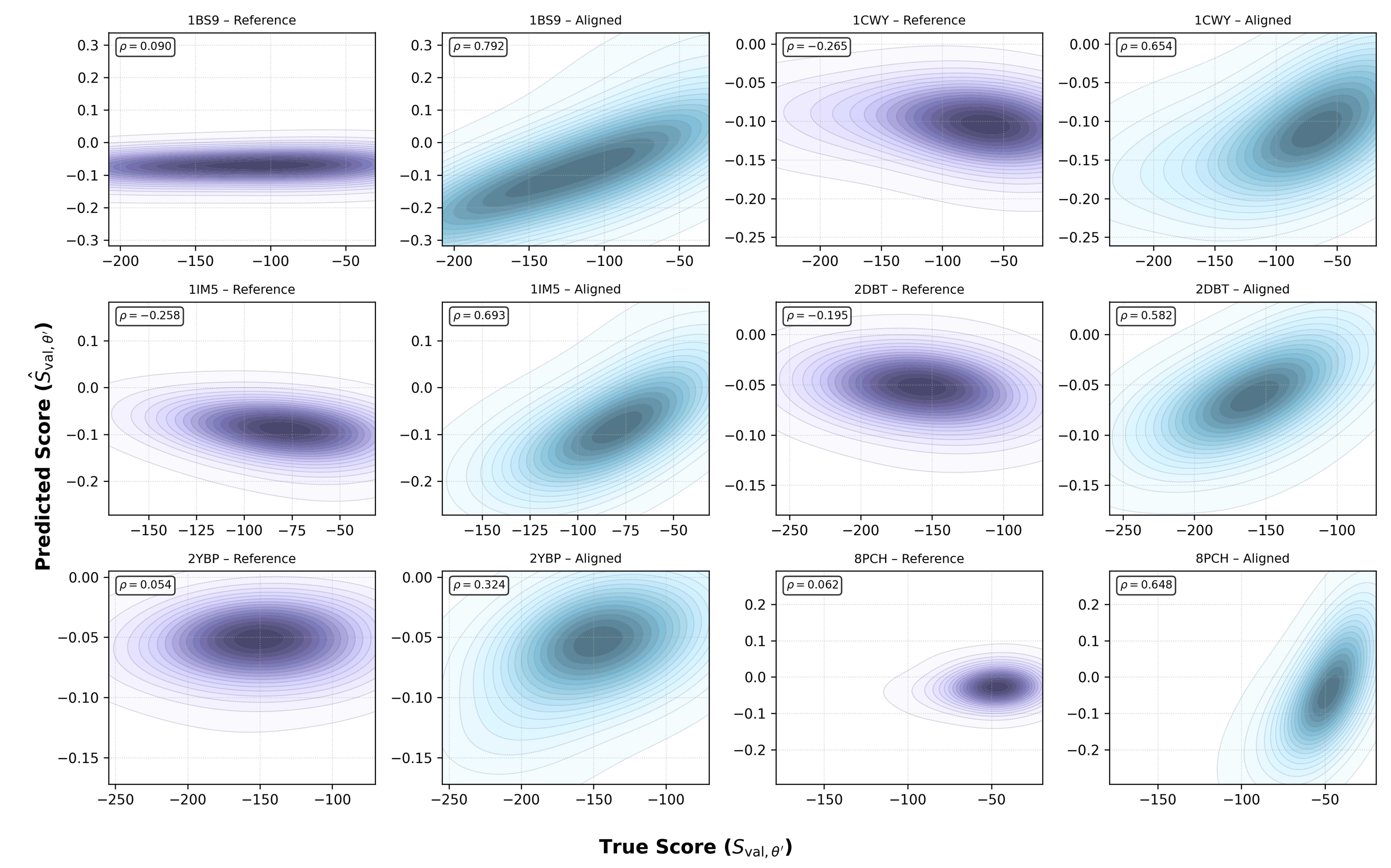
These are the same six tasks used to construct the alignment preferences. The result establishes task-specific score calibration, not transfer to new enzymes or measured catalytic activity. A confident fold with the requested geometry is a useful computational filter, but it is not an activity assay.

Constructing preferences and the D2-DPO objective Aside

For each enzyme, we use 16 prompts and generate 128 candidates per prompt: 2,048 candidates per task. Designs span 200–600 residues, with active-site identities, geometry, and inter-site distances constrained.

The external objective has the form

$$s_{\mathrm{ext}} = a\log(\mathrm{pTM}) - \frac{\mathrm{cRMSD}}{\tau},$$

where $a$ and $\tau$ set the relative weight and scale of the two terms. Higher fold confidence and smaller geometric error are preferred. We rank within-batch candidate pairs by their score gaps and retain the largest gaps for alignment.

Let $\theta_{\mathrm{ref}}$ denote the pretrained model and $\theta$ the aligned model. Define the sequence-denoising improvement at a sampled corruption time by

$$D_\theta(z_0,z_t) = \widehat{\mathcal L}_{\mathrm{seq},t}^{\theta_{\mathrm{ref}}}(z_0,z_t) - \widehat{\mathcal L}_{\mathrm{seq},t}^{\theta}(z_0,z_t).$$

For winner and loser candidates, $w$ and $l$, the training loss is

$$\mathcal L_{\mathrm{D2\text{-}DPO}} = -\mathbb E\log\operatorname{sigmoid} \left( \kappa\left[D_\theta(w_0,w_t)-D_\theta(l_0,l_t)\right] \right).$$

This rewards a larger improvement over the reference model on preferred candidates than on dispreferred ones. The update targets the sequence reverse process; structure and the other tracks supply conditioning information.

The reported evaluation measures rank agreement with the computational score. It does not measure a change in the fraction of experimentally functional designs. The next distinct questions are whether the preference transfers to new tasks and whether it improves the candidates that matter in an experiment.

Connecting models and experiments

The enzyme example begins with an unusually precise instruction: keep these residues in this arrangement. Many of the biological tools we want to build will require more than that. We will need to specify combinations of properties, understand which constraints conflict, and learn from the cases where a plausible design does not work.

Odyssey gives us a way to put sequence and geometry inside the same design process, train that process at substantial scale, and adjust its preferences toward a chosen objective. The important next step is making those objectives increasingly faithful to the behavior we want from the molecule. That is where our modeling work and experimental platform meet: experiments can test the properties that a model currently only approximates, and supply the evidence needed to improve those approximations.

We want the instructions we can give a protein model to become much closer to the instructions we would give an engineer. This release develops the model on which we can begin to do that.

Responsible development Aside

Protein models are dual-use. Our work is informed by the Principles for the Responsible Development of AI for Biological Design. We support the continued development of capability evaluations, screening standards, and access norms as the field advances. We believe publishing the methods and evidence in this release has benefits that outweigh its risks.

The paper contains the full methods and supplementary experiments. The implementation is available on GitHub.